

1. Introduction
2. Experimental Procedure
2.1. Materials and specimens
2.2. Stress measurement using characteristic X-ray CrKα
2.3. Stress measurement using high-energy SR
2.4. X-ray penetration depth and measured stress value
2.5. Measurement of X-ray elastic constants
3. Results and Discussion
3.1. Stress distribution under the surface of shot peening
3.2. X-ray elastic constants
3.3. Non-destructive measurement of residual stress in shot peened materials
3.4. Stress values calculated by the linear approximation of the sin2ψ method
4. Conclusion
1. Introduction
The X-ray diffraction method is widely used as a nondestructive method for measuring the residual stress of crystalline materials. In particular, it has been established as a field technique for controlling residual stresses introduced by heat treatment or surface treatment of steel materials.1,2,3,4,5,6) However, the usual X-ray method uses a chrome tube, and the penetration depth of the X-ray beam is only a few micrometers. Therefore, in order to obtain the residual stress distribution extending over an area of several hundred micrometers introduced by shot peening, laser peening, and water jet peening, which are important for improving fatigue strength, the surface layer has been removed by electropolishing and repeated measurement has been used. The residual stress measured by this sequential surface removal method requires correction for surface removal, is time-consuming, and is not a nondestructive method in the strict sense.
Neutron stress measurement is attracting attention as a method for measuring the inside of materials to compensate for the disadvantage of the X-ray method, which measures stress in an extremely thin surface layer.7,8,9) Neutron stress measurement is based on the principle of diffraction of crystals as in the X-ray method, and its depth of penetration is about 1,000 times greater than that of X-rays, making it suitable for measuring the interior of materials. However, since the intensity of the neutron source is not strong, the measurement area must be larger than a few millimeters, and the spatial resolution of the measurement is low. In addition, since some of the neutrons escape to the surface near the surface, it is necessary to compensate for the surface effect caused by the irradiation volume. Therefore, there is a limitation in determining the stress distribution in the region of several hundred micrometers on the surface treated material.
On the other hand, a third-generation synchrotron radiation (SR) facility, produces high-energy X-rays of arbitrary wavelength with high brightness and high directionality. The higher the energy, i.e., the shorter the wavelength, the greater the penetration depth of X-rays. Therefore, high-energy X-rays are of interest as a stress measurement method that fills the gap between conventional tube-type laboratory X-ray measurements and neutron measurements.
However, the X-ray detector itself is also easily penetrated, which lowers the detection efficiency and makes X-ray shaping difficult, making handling difficult. In addition, diffraction lines at high angles with high strain sensitivity suitable for stress evaluation usually have high order diffraction, and since the atomic scattering factor governing the X-ray diffraction intensity is a function of sinθ/λ (θ: diffraction angle, λ: wavelength), the signal intensity becomes significantly low.10,11,12,13,14) Therefore, it is necessary to use low-angle diffraction lines with relatively high diffraction strength. For this reason, energy-dispersive X-ray diffraction has been used in conventional stress evaluations using high-energy SR.15,16,17) However, the accuracy of stress measurement by energy diffraction is not sufficient at present. On the other hand, monochromatic X-rays are also used, but the sin2ψ method is not used and the measurement accuracy is not sufficient.18,19)
Therefore, in this study, we examined a stress measurement method using the sin2ψ method with monochromatic high-energy X-rays (30~72 keV). Using carbon steel for mechanical structures as the experimental material, we investigated a method for evaluating the stress-free fracture in the deep part of the material using high-energy SR under two different conditions of shot peening and different distributions of residual stress.
2. Experimental Procedure
2.1. Materials and specimens
The experimental material was carbon steel for mechanical construction (SM45C). After forming the test specimens, they were annealed at 850 °C for 1 h before shot peening. The yield point of the material is 319 MPa and tensile strength is 583 MPa. The test specimen is 4 mm thick and the shot surface is 10 × 56 mm.
A suction-spray type shot peening machine was used for the shots. Cast steel with a hardness of HV = 400 was used for the shots. The unquenched test specimens were shot peened under the two conditions shown in Table 1. The test specimen peened with 0.4 mm particles is called the MP (moderately peened) test specimen (test specimen No. 1) and the one peened with 0.8 mm particles is called the HP (heavily peened) test specimen (test specimen No. 2).
Table 1.
Shot-peening conditions.
| Condition |
Nominal shot diameter (mm) |
Air pressure (atm) |
Coverage (%) |
|
Medium peening (MP) Specimen No.1 | 0.4 | 1.5 | 100 |
|
Heavy peening (HP) Specimen No.2 | 0.8 | 3.0 | 100 |
Table 2.
X-ray conditions for stress measurement by Cr-Kα radiation.
2.2. Stress measurement using characteristic X-ray CrKα
A laboratory X-ray machine (Mc Science: MXP18) was used to measure the residual stress distribution under the surface of the shot peening test specimen by the parallel beam of Cr-Kα radiation. Table 2 shows the conditions for stress measurement.
The stress measurements were repeated while the surface layer was removed by successive electrolytic polishing using the parallel tilt method. In the sin2ψ method, measurements were made in 0.1 increments from 0 to 0.5, and the peak position was determined by the semi-valent midpoint method according to the standard. The stresses were obtained by multiplying the linearly approximated gradient M of the sin2ψ diagram by the stress constant K.
The stress constant K is a function of the following X-ray elastic constants.
where E is the X-ray Young’s modulus and ν is the X-ray Poisson’s ratio. The values used are the standard values20) and are shown in Table 2.
2.3. Stress measurement using high-energy SR
The high-energy X-ray stress evaluation experiment was conducted on the beamline BL02B1.21) This beamline is equipped with a high-energy X-ray beam with energies from 17 to 72 keV and a highly accurate multi-axis goniometer. Fig. 1 shows a schematic layout of the diffractometer used in the experiment. When high-energy X-rays are used, the Bragg angle of the diffraction line that can be measured becomes small14) and when the parallel tilt method is used as the stress measurement method, the measurement range of sin2ψ becomes narrower.
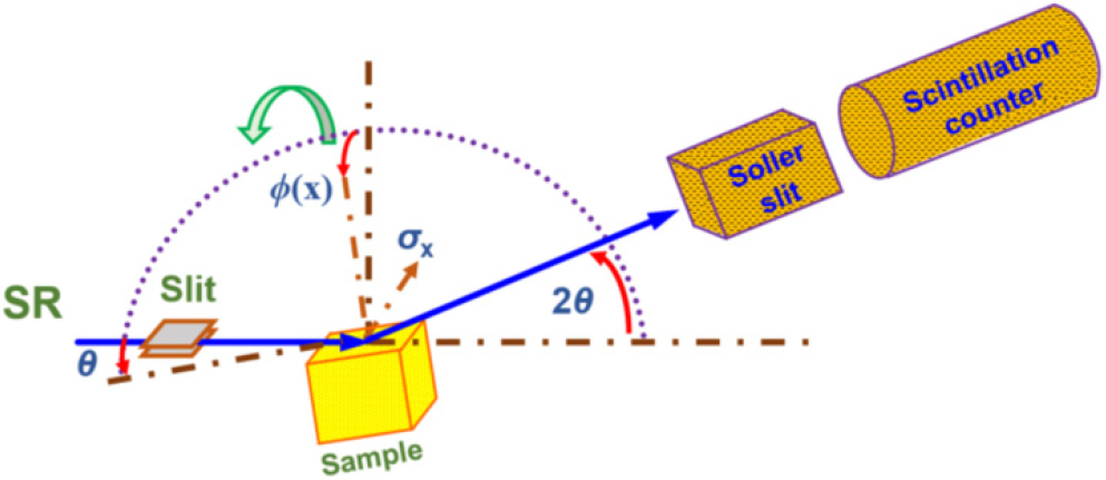
Therefore, the side tilt method (constant ψ method) was adopted as the X-ray stress measurement method. The X-ray beam irradiating the sample was aligned to a height of 0.5 mm × width of 2.0 mm using a four-quadrant slit, and a scintillation counter detector was used to detect the diffraction lines to remove the influence of fluorescent X-rays and other sources. A long solar slit with a resolution of 0.03° and a length of 500 mm was placed in front of the detector.
The emitted light used in the measurement was monochromatized using a Si(311) two-crystal spectrometer, and its parallelism and monochromaticity are extremely high compared to the tube-type X-ray source used in the laboratory system. Therefore, even if the crystal grain size of the sample is small enough not to be a problem in the laboratory system, a slight waviness may be observed in the sin2ψ diagram, which should be a straight line, due to the high quality of the emitted light. Therefore, in this experiment, the sample was rotated around the φ axis (in the sample plane) at a speed of about once per second while the measurement was performed.
Since the diffraction lines with relatively small Bragg angle are used in this experiment, the amount of diffraction line shift is small in relation to the change of ψ angle, and the misalignment between the center of rotation of the goniometer and the measurement point is a problem of measurement accuracy in the stress evaluation. Therefore, while rotating the sample around the ψ-axis and around the axis normal to the sample surface (φ-axis), the sample surface was observed with a light microscope, and the measurement site on the sample surface and the center of rotation of the goniometer were matched with an accuracy of about ±10 µm.
Table 3 shows the conditions for stress measurement. Three types of X-ray energy levels were used: 30, 60, and 72 keV. The diffraction planes used were 321 and 633, 552, and 721, which were strong diffraction planes calculated in advance by Rietveld simulation RDETAN.22,23) Here, when the strain is zero, the latter three diffraction plane intervals are equal and the diffraction angles are equal.
Table 3.
X-ray conditions for stress measurement by synchrotron radiation.
| X-ray energy (keV) | 30 | 60 | 72 | ||
| Diffraction | 321 | 721* | 321 | 321 | 721* |
| Diffraction angle (deg.) | 31.25 | 63.88 | 15.91 | 12.87 | 25.43 |
| Preset time (sec) | 2 | 20 | 1 | 2 | 10 |
| Scan speed (deg./min) | 0.3 | 0.03 | 0.3 | 0.06 | 0.018 |
The diffraction curves for 633, 552, and 721 diffractions were approximated by a Gaussian function as one profile, and the peak position was taken as the diffraction angle. The same applies to 321 diffraction.
2.4. X-ray penetration depth and measured stress value
The X-ray intensity of a material decreases exponentially with the transmission distance × as it passes through the material. If the incident X-ray intensity is I0, the transmitted X-ray intensity is expressed by the following equation using the linear absorption coefficient µ of the material.1,11)
If the effective penetration depth T is the vertical depth from the surface where the X-ray intensity ratio I/I0 becomes 1/e, it can be expressed by the following equation for the side inclination method.1)
In addition, for the inclination method,
Here, θ0 is the distortion-free diffraction angle, and ψ is the inclination angle of the side inclination method. When ψ = 0, the penetration depth is the same for both and is given by the following Eq. (6).
Table 4 summarizes the depth of penetration with respect to the linear absorption coefficient µ and T0 for each diffraction.
Table 4.
Penetration depths of X-rays.
|
Energy (keV) |
Linear absorption coefficient µ (cm-1) | Diffraction |
Penetration depths T0 (µm) |
| 5.41* | 889 | 211 | 5.51 |
| 30 | 63.64 | 321 633, 552, 721 | 21.2 41.6 |
| 60 | 9.272 | 321 | 74.6 |
| 72 | 5.902 | 321 633, 552, 721 | 94.9 186 |
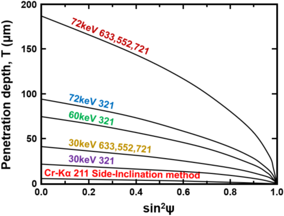
Fig. 2 shows the relationship between T and sin2ψ. Here, the case of the Cr-Kα radiation shows the depth of penetration by the translational method, and the other cases by the side tilt method. The value of T0 is 5.5 µm for the Cr-Kα radiation, while the maximum value is 186 µm for 72 keV, which is 34 times deeper.
The stress value measured by X-rays is the weighted average stress value expressed by the following equation using the stress distribution σ(z), where h is the thickness of the sample.1,24,25,26)
2.5. Measurement of X-ray elastic constants
The X-ray elastic constants were measured by obtaining a sin2ψ diagram under four-point bending loading and determining the slope with respect to the applied stress and the rate of change of the intersection point with the vertical axis with respect to the applied stress. The test specimen used in this experiment was 2 mm thick, 10 mm wide, 56 mm long, and was left unburned. The inner span of the pin is 10 mm and the outer span is 36 mm in 4-point bending. A strain gage was attached to the compression side and monitored to obtain the sin2ψ diagram at each set strain.
3. Results and Discussion
3.1. Stress distribution under the surface of shot peening
The residual stress distribution measured by Cr-Kα radiation is shown in Fig. 3. The surface residual stress is compressive, and the depth of the region where the residual stress is distributed, z0 is 150 µm for the MP specimen and 300 µm for the HP specimen.
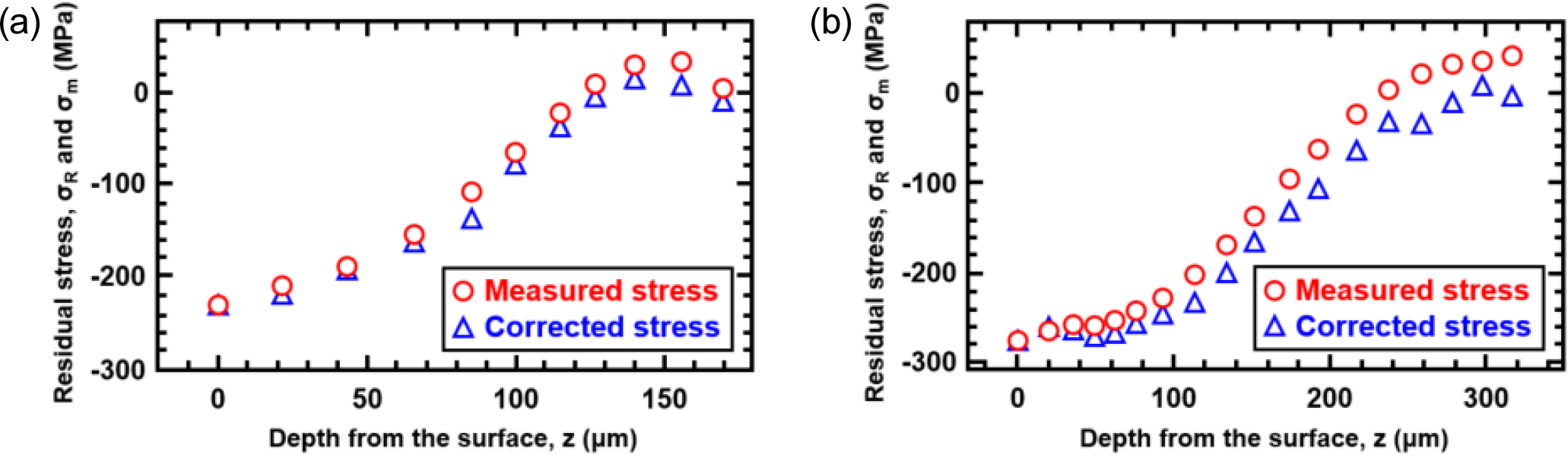
The larger the shot diameter, the deeper the penetration.27) Since the shot peening does not affect the residual stress above the depth of z0, the residual stress is considered to be zero.
From the measured residual stress obtained by the sequential surface layer removal method, the effect of surface removal was corrected using the following equation.28)
where σm(z) is the stress measured at the surface layer z by the sequential surface layer removal method, σR(z) is the corrected stress, and h is the plate thickness. The residual stress value after correction is indicated by a red circle. The residual stress after correction is indicated by a red circle. The measured stress inside the residual stress-damped area is set to zero to obtain the corrected stress. In the corrected residual stress distribution, there is tension balancing the surface compression.
3.2. X-ray elastic constants
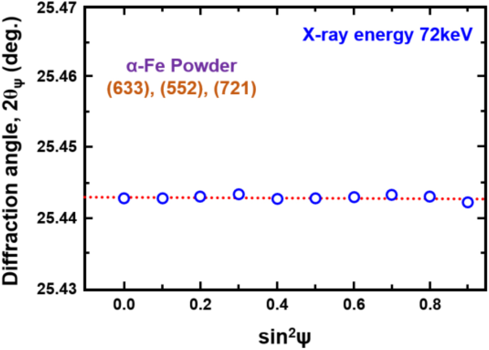
In order to confirm the alignment of this optical system with SR, we measured the stress by the sin2ψ method using iron powder as a sample. As shown in Fig. 4, the diffraction angle does not change in a wide range of sin2ψ and the stress value can be regarded as zero. This confirms that the alignment of the optical system has been achieved.
Since the SR measurement is different from the laboratory measurement in that it utilizes low-angle diffraction, the measurement of the X-ray elastic constants was used to determine the accuracy of the measurement. It is also known that the X-ray elastic constants generally depend on the diffraction plane. Therefore, in the evaluation of X-ray stress, it is desirable to use diffraction lines containing only contributions from a single diffraction plane. However, in experiments using high-energy X-rays, it is necessary to use diffraction lines including contributions from multiple diffraction planes, considering the intensity, angle, and separation of the diffraction lines. In this experiment, the diffraction angles of 633, 552, and 721 were used, and these multiple diffractions were considered as one diffraction to measure the X-ray elastic constants. The X-ray energy was 72 keV, which is a low angle of diffraction.
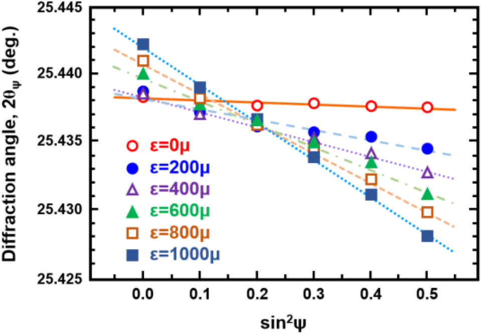
Fig. 5 shows the sin2ψ diagram obtained for each load strain. A linear approximation is almost established in the range of sin2ψ = 0 to 0.5, and the regression line is shown in the figure. Fig. 6 shows the variation of the slope M of the straight line and the intercept 2θψ=0 with the vertical axis as a function of the applied stress. Here, the negative stress value is the value at the surface of the bending test specimen obtained by multiplying the applied strain by the mechanical elastic constant EM = 211.4 GPa. The regression line that is a linear approximation of the relationship in Fig. 6 is shown in the figure. Here, in the relationship between the specimen and loading stress, a linear approximation was made for loading stresses above 80 MPa. In the case of the measurement at a loading stress lower than 80 MPa, it is considered that there was a shift in the diffraction angle during strain loading, and thus, it was excluded from the linear approximation.
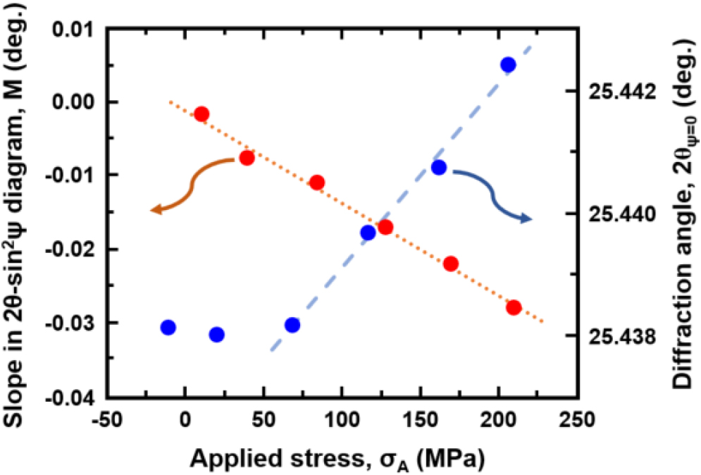
The X-ray elastic constant is usually determined by the following formula from the rate of change of the slope of the sin2ψ diagram and the intercept with the vertical axis with respect to the applied stress.1)
However, when determining the tilt M and the slice <2θ>ψ=0 for each stress value σA from the measured sin2ψ diagram, it is expected to be affected by the stress distribution in the depth direction of the 4-point bend test specimen due to the high X-ray energy of 72 keV and the depth of penetration in this experiment. In this case, the slope and intercept are obtained by linear approximation using Fig. 5, and the x-ray elastic constants are obtained using Eq. (9). For this reason, as described in the section 3.4, we evaluated the x-ray elastic constants for the nonlinear relationship between sin2ψ and <2θ>, assuming that the data points for every 0.1 increment of sin2ψ from 0 to 0.5 are linearly approximated by the least-squares method [Eq. (20), described below]. Fig. 6 shows that the x-ray elastic constants evaluated by this method are E/(1+ν) = 173.2 GPa and ν = 0.363.
On the other hand, as a simple calculation method, as described in the section 3.4, in a uniaxial stress state, the stress obtained by linear approximation in the measurement range of sin2ψ from 0 to 0.5 is the stress value measured at a penetration depth T0.3 = 155.6 µm when sin2ψ = 0.3. If the stress on the surface is σ0, the load stress measured by X-ray is σA = 0.8444σ0. Using this relationship, the X-ray elastic constant is obtained from Eq. (9). Then, E/(1+ν) = 174.3 GPa, ν = 0.356. This value is almost the same as that obtained when the nonlinearity of the sin2ψ diagram is strictly taken into account.
The X-ray elastic constants calculated from the single crystal elastic constants29) shown in Table 5 using the Kroner model30) are shown in Table 6.
Table 5.
Elastic constants of iron single and polycrystals.
| Single crystal | Poly crystal | ||||
|
C11 (GPa) |
C12 (GPa) |
C44 (GPa) |
EM (GPa) | νM |
EM/(1+νM) (GPa) |
| 228.0 | 132.0 | 116.5 | 211.4 | 0.285 | 164.5 |
Table 6.
X-ray elastic constants of iron poly crystals calculated by Kroner’s model.
| hkl | Intensity ratio |
Ex/(1+νx) (GPa) |
Ex (GPa) | νx |
| 321 | 100 | 175.5 | 223.4 | 0.273 |
| 633 | 4.85 | 175.5 | 223.4 | 0.273 |
| 552 | 4.85 | 183.5 | 232.0 | 0.264 |
| 721 | 9.70 | 143.9 | 188.4 | 0.309 |
The table also shows the diffraction intensity ratios obtained by Rietveld simulation.22,23) The orientation coefficient of the 321 diffraction is the same as that of the 211 diffraction adopted in the X-ray standard, and the calculated value is also equal to E/(1+ν) = 175 GPa. On the other hand, the X-ray elastic constants of the 633, 552, and 721 diffractions are different from each other. Here, if the weight of the intensity ratio is multiplied and the average value is taken, the calculated value becomes E/(1+ν) = 162 GPa, which is very close to the value measured above. This suggests that a low diffraction angle is used for SR. Since the diffraction grating is parallel, the strain sensitivity is low, but the incident beam is parallel and strong, and the accuracy of the recorder is higher than that of a normal laboratory diffractometer, so it can be concluded that stress measurements can be performed with sufficient accuracy. In the calculation of stress using the sin2ψ method in the next section, the measured value E/(1+ν) = 173 GPa for 633, 552, and 721 diffractions and the standard value E/(1+ν) = 175 GPa for 321 diffractions were used, and the stress constant calculated from Eq. (2) was used to determine the stress value from the linear gradient of the sin2ψ diagram.
On the other hand, the measured Poisson’s ratio is larger than the calculated value. As shown in Fig. 6, this is considered to be due to the fact that a sufficient number of measurement points have not been obtained due to the deviation of the diffraction angle, and further re-measurement will be necessary.
3.3. Non-destructive measurement of residual stress in shot peened materials
Residual stress was measured using the sin2ψ method with three different energies for test specimens that had been subjected to two types of shot peening. The sin2ψ diagram for the MP test specimen with X-ray energy of 72 keV and 321 diffraction is shown in Fig. 7.
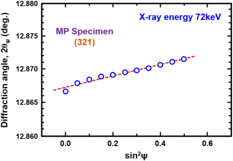
Although the amount of shift in the diffraction line due to residual stress is small because the diffraction angle is relatively low, a good linear relationship is shown in the sin2ψ range from 0 to 0.5. The residual stress was evaluated from the slope of the regression line. Similar measurements were also performed on the HP test specimen.
Tables 7 and 8 show the results of stress evaluation at five penetration depths, which were changed by the diffraction line and X-ray energy used, for two types of test specimens.
Table 7.
Residual stress determined from sin2ψ method for MP specimen.
| Energy (keV) | Diffraction | Residual stress (MPa) |
| 30 |
321 633, 552, 721 |
-281 ± 19 -242 ± 14 |
| 60 | 321 | -129 ± 18 |
| 72 |
321 633, 552, 721 |
-117 ± 7, -132 ± 11 -27 ± 4 |
The 68.3 % confidence limit is also shown in the table, but the linear approximation is almost valid. The stress value observed in this experiment is the weighted average value with the penetration depth of Eq. (6) as a parameter. The residual stress obtained by the sin2ψ method is equi-biaxial, and is considered to correspond to the penetration depth of T0 (constant) as described in the section 3.4. Next, to facilitate the comparison of the results of this experiment with those obtained by the sequential surface removal method, the evaluation value (integral stress value) for the penetration depth T was calculated using Eq. (7) using the residual stress distribution after correction in Fig. 3.
In Fig. 8, the experimental results in Tables 7 and 8 are plotted at the T0 position along with the calculated values.
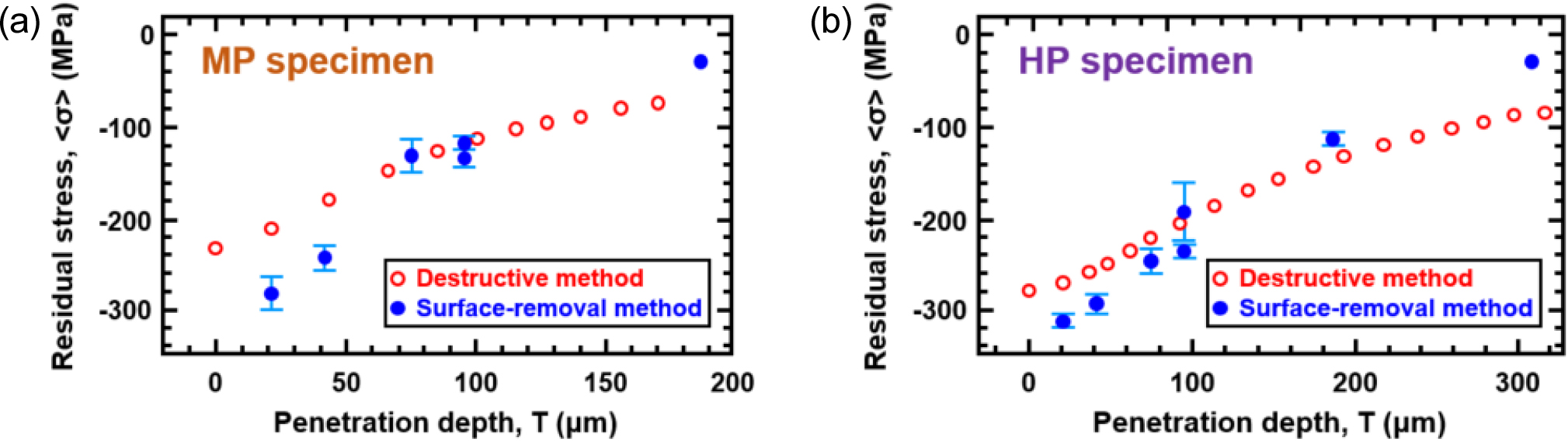
Table 8.
Residual stress determined from sin2ψ method for HP specimen.
| Energy (keV) | Diffraction | Residual stress (MPa) |
| 30 |
321 633, 552, 721 |
-310 ± 7 -290 ± 10 |
| 60 | 321 | -243 ± 14 |
| 72 |
321 633, 552, 721 |
-233 ± 9, -189 ± 31 -111 ± 5 |
The values measured nondestructively using high-energy X-rays are slightly larger at shallower penetration depths and slightly lower at deeper penetration depths compared to the sequential surface removal method, but overall there is good agreement. From this, it can be concluded that this X-ray stress evaluation method using high-energy SR X-rays is effective as a nondestructive measurement method.
In the discussion up to this point, we have assumed a plane stress state inside the sample. However, when X-rays with a deep penetration depth are used, as in the present experiment, it is possible that the plane stress state is not established inside the sample. For this reason, we next consider the case of a triaxial stress state. Assuming a coordinate system with the z-axis perpendicular to the sample surface and the x- and y-axes perpendicular to this axis, and assuming that the principal stress values are σ1, σ2, and σ3, respectively, the basic stress equation is given by Eq. (10).
When the sample is rotated around the φ axis during measurement, as in this experiment, the average is taken for the φ axis, and (σ1+σ2)/2 is newly set as σ1, which gives Eq. (11).
The stress value calculated from the slope of the sin2ψ diagram indicates the stress value σ1-σ3 in the specimen surface, not σ1. Therefore, the experimental results using SR shown in Fig. 8 may include the effect of σ3, but the effect is considered to be relatively small compared to the results obtained by the sequential surface removal method. This suggests that σ3 inside the specimen is almost 0 at the X-ray penetration depth in this experiment, and indicates that the results of this report, which assume a plane stress state, are effective as a first approximation of the nondestructive stress evaluation value. However, analysis and experiments that consider a triaxial stress state are likely to be important for nondestructive stress evaluation using high-energy SR, and we would like to conduct detailed studies in the future. In addition, when there is a stress gradient inside the X-ray penetration depth, nonlinearity appears in the sin2ψ diagram, and a method has been proposed to analyze the residual stress distribution based on the analysis of this nonlinearity,24,25,26) but we will also consider this method in the future.
3.4. Stress values calculated by the linear approximation of the sin2ψ method
When there is a stress gradient in the X-ray penetration depth, the relationship between the diffraction angle and sin2ψ is non-linear. However, in this case, the usual linear approximation is performed and the stress value obtained by multiplying the slope of the line by the stress constant is examined to determine the stress at which penetration depth. Here, we consider the case where the diffraction angle is measured by the sin2ψ method from 0 to 0.5 in steps of 0.1. The stress is assumed to be uniaxial or equi-biaxial, and the distribution in the depth z direction is given by the linear distribution in the following equation.
For example, when a bending stress is applied to a flat plate of height h, the surface stress is σ0, which becomes Eq. (13).
Then, Eq. (10) can be substituted into Eq. (7) to obtain Eq. (14).
where h is assumed to be sufficiently large compared to T. Assuming that the measured diffraction angle is a weighted average of the penetration depth, the following equation holds.
where ν' is ν for uniaxial stress and 2ν for equi-biaxial stress. Here, <σ> is the measured stress given by Eq. (14). Substituting Eq. (14) into Eq. (15), we obtain the following Eq. (16).
Here, we used Eq. (17), which is the depth of penetration for the side inclination method.
When the stress gradient cannot be ignored, the relationship between x = sin2ψ and y = <2θ> obtained by Eq. (9) becomes nonlinear. When this nonlinear relationship is evaluated by linear approximation using the least squares method with the <2θ>i values calculated by Eq. (13) as data points for xi from 0 to 0.5 in increments of 0.1, the slope M and intercept <2θ>ψ=0 are calculated by the following equation.
If we find M and <2θ>ψ=0 in the above equation, we get Eq. (19).
By substituting A = -2/h, ν' = ν, which are the 4-point bending cases, into the above equation and calculating by substituting the experimental conditions of 633, 552, and 721 diffraction, Eq. (20) can be obtained.
The above formula is used for evaluation of the X-ray elastic constant, taking nonlinearity into consideration. On the other hand, the relationship between the diffraction angle and sin2ψ measured by the sin2ψ method in 0.1 increments from 0 to 0.5 is approximated by a straight line as in the usual case, and the stress value obtained by multiplying the slope of the straight line by the stress constant is given by the following equation.
Here, we use ν = 0.285, which becomes Eq. (22) for the uniaxial stress state.
In the equi-biaxial stress state, Eq. (23) is obtained.
Comparing these equations with Eqs. (12) and (14), the uni-axial stress state measures a stress of approximately sin2ψ = 0.3. On the other hand, the equi-biaxial stress state corresponds to a penetration depth of sin2ψ = 0.06. Although this depth depends on the stress distribution and cannot be determined in general, in this study it is assumed that the residual stress is measured at the depth corresponding to T0 because shot peening is performed in the equi-biaxial stress state. The ratio of T0 to T0.3 is 0.8367.
4. Conclusion
Using monochromatic high-energy X-rays (30, 60, 72 keV) obtained from a large radiolucent facility, a stress measurement method was developed by the sin2ψ method and applied to the non-destructive measurement of residual stresses beneath the surface of shot-peened carbon steel. The nondestructive measurements using high-energy X-rays were compared with the residual stress distributions measured by the conventional sequential surface removal method using laboratory X-rays. The conclusions obtained are as follows;
(1) The diffraction angles of high intensity by high-energy X-rays are low, but can be measured with sufficient accuracy.
(2) Stress measurement is possible by analyzing the three diffraction profiles 633, 552 and 721 as one diffraction profile. The measured linear elastic constants are close to the weighted average of the intensity ratios of the elastic constants of single crystals obtained by the Kroner model.
(3) The experimental results of high-energy X-ray stress evaluation using SR are in good agreement with those obtained by the sequential surface removal method, and it is confirmed that this evaluation method is useful as a nondestructive stress evaluation method for deep materials.
