Development of Gas Sensors for Measuring Gas Emission and Diffusion Coefficient in Gas Charged EPDM Polymer Using Volumetric and Manometric Analysis

Ji Hun Lee; Sang Koo Jeon

doi:10.3740/MRSK.2025.35.3.127

Preview

Research Paper

Korean Journal of Materials Research. 27 March 2025. 127-138
https://doi.org/10.3740/MRSK.2025.35.3.127

Development of Gas Sensors for Measuring Gas Emission and Diffusion Coefficient in Gas Charged EPDM Polymer Using Volumetric and Manometric Analysis

Ji Hun Lee¹^†

Sang Koo Jeon¹

¹Hydrogen Energy Group, Korea Research Institute of Standards and Science, Daejeon 34113, South Korea

^†Corresponding author E-Mail : ljh93@kriss.re.kr (J. H. Lee, KRISS)

License (open-access, https://creativecommons.org/licenses/by-nc/4.0/):

This is an Open-Access article distributed under the terms of the Creative Commons Attribution Non-Commercial License (https://creativecommons.org/licenses/by-nc/4.0/) which permits unrestricted non-commercial use, distribution, and reproduction in any medium, provided the original work is properly cited.

ABSTRACT

Gas sensors are crucial devices in various fields including industrial safety, environmental monitoring, gas infrastructure and medical diagnosis. These sensors measure specific gases in different environments, guaranteeing operational safety and efficiency through precise on-site measurements. Designed for high sensitivity, stability and reliability, gas sensors must also be cost-effective, quickly responsive and compact. To address these diverse requirements, we have developed two types of gas sensors based on the volumetric and the manometric method. These sensors operate by measuring the gas volume and the pressure changes, respectively, of the emitted gas. These sensors are capable of determining gas transport parameters such as gas uptake, solubility and diffusion coefficient for gas-charged polymers in high pressure environment. The sensors provide rapid responses within one second and can measure gas concentrations ranging from 0.01 wt ppm to 1500 wt ppm with adjustable sensitivity and measurement ranges. Performance evaluations demonstrate the sensors' reliability, adaptability to varying measurement ranges and stability under temperature and pressure fluctuations. As a result, this sensor system facilitates the real time detection and analysis of gas transport properties in pure gases including H₂, He, N₂, O₂ and Ar, making it suitable for pure gas sensing.

Keywords

gas sensors

volumetric measurement

manometric measurement

gas uptake

diffusion

MAIN

1. Introduction
2. Experimental Procedure
2.1. Specimen preparation and high-pressure gas charging
2.2. Volumetric measurement of the released gas from charged polymers
2.3. Manometric measurement of the released gas from charged polymers
2.4. Analysis program for obtaining transport parameters
3. Results and Discussion
3.1. Volumetric measurement
3.2. Manometric measurement
3.3. Performance comparison between volumetric and manometric gas sensors
4. Conclusion

1. Introduction

Gas sensors are crucial devices in various fields such as industrial safety, environmental monitoring, gas infrastructure and medical diagnosis. They are essential for ensuring safety, particularly under environments where hazardous gases like hydrogen or carbon monoxide are released.^{1,2,3,4,5,6,7,8,9,10)} Early detection of gas emissions and leaks can prevent accidents, fires and other risks. It is also essential for environmental monitoring, as it helps detect pollutants and maintain air quality. Accurate gas sensing plays an important role in optimizing operations, particularly for renewable energy source like hydrogen. By ensuring precise monitoring of hydrogen gas concentrations, it enhances safety, efficiency and performance throughout the hydrogen production, storage and distribution processes.^{11,12,13,14,15,16,17,18,19,20,21,22)}

In hydrogen refueling station charged to high-pressure H₂, polymer materials play an important role.^{23,24,25,26,27,28,29,30,31,32,33,34,35,36,37,38,39,40,41,42,43,44,45)} For instance, polymer-based materials such as O-ring seals, gasket, liner material and non-metallic pipeline are widely used. It was designed to withstand hydrogen environments. However, these polymers are subjected to harsh conditions including wide temperature fluctuations (-70 °C to 90 °C) and pressure variations (1 MPa to 90 MPa). These conditions can lead to seal damage, insufficient contact with glove and gas permeation through polymer seals, all of which can result in hydrogen leakage.^{46,47,48,49,50,51,52)}

Gas permeation, including hydrogen permeation, in polymer materials also occurs when gases pass through the polymer matrix due to diffusion. This process is influenced by various factors, including temperature, pressure and chemical nature of both the gas and the polymer.^53,54,55) For instance, in the use of polymer membranes for gas separation, materials like polyimide are employed to selectively permeate gases like oxygen or carbon dioxide while blocking other gases. A common example is the use of polymeric membranes in CO₂ capture systems, where the membrane’s permeability to CO₂ is crucial for effective separation from industrial emissions. However, the permeation rate can vary based on the polymer’s structure, with amorphous polymers typically having higher permeability compared to crystalline ones. Gas permeation is a key consideration in applications like gas storage and delivery, where polymers need to have low gas diffusion/permeability to avoid leakage and maintain system integrity.

Meanwhile, gas sensors are vital for accurately detecting specific gas concentration and leakage across applications where gas is produced, stored and used, such as fuel cells, storage facilities and transportation systems.^56,57) These gas sensors are developed based on different sensing principles, each with its own advantages and limitations. Infrared (IR) gas sensing^58,59,60) works on the principle that gas molecules absorb infrared light at specific wavelengths. The intensity of the absorbed light is measured and correlated to concentration of the corresponding gas. The main advantages of IR gas sensing include high sensitivity, selectivity and ability to detect gases over a wide range of concentrations. However, it can be affected by environmental conditions including temperature and humidity and may require regular calibration for accurate measurements.

Semiconductor gas sensors^61,62,63) operate based on the principle that gas molecules interact with the surface of a semiconductor material (typically metal oxides), causing a change in its electrical resistance. The change in resistance is measured and intercorrelated to the concentrations of the target gas. The advantages include low cost, fast response and small size. However, they can be influenced by factors like temperature, pressure and humidity and may exhibit cross-sensitivity to other gases, reducing accuracy.

Catalytic combustion gas sensors^64,65,66) operate by detecting gases through the catalytic oxidation of the target gas on a heated catalyst surface, which generates heat. This heat change is measured and used to determine the gas concentration. The advantages include high sensitivity to combustible gases and reliability in detecting flammable gases at low concentrations. However, they have a limited lifespan, especially in the presence of contaminants like silicone or lead. These sensors may require regular maintenance to ensure the accurate performance.

An optical spectroscopy gas sensor^67,68,69) operates based on the principle that gas molecules absorb or emit light at specific wavelengths. When light passes through a gas sample or is reflected from it, the gas molecules absorb light at characteristic absorption bands corresponding to their molecular structure. The amount of absorbed light is then measured, which is correlated to concentrations of the gas. Key features of optical spectroscopy gas sensors include high sensitivity, non-destructive measurement and ability to detect low concentrations of gases with high accuracy. These sensors are capable of detecting wide ranges of gases and are immune to interference from most other substances. However, they may be affected by environmental factors such as temperature, pressure and the presence of other gases in complex mixtures.

An electrochemical gas sensor^70,71,72) operates by detecting gases through a chemical reaction between the target gas and the electrodes in an electrolyte. This reaction produces an electrical current proportional to concentrations of the gas, which is then measured and used to determine the gas level. The advantages of electrochemical sensors include high sensitivity, low power consumption, and good selectivity for specific gases. However, they can be influenced by factors like temperature and humidity and their lifespan may be limited due to the degradation of the electrodes or electrolyte over time.

Finally, gas chromatography^{73,74,75,76,77,78,79)} and mass spectrometry^80,81,82) provide highly precise analysis and are commonly used in research and laboratory settings. Gas chromatography separates and analyzes individual components in gas mixtures, while mass spectrometry identifies gas molecules based on their mass after ionization. However, these sensing systems are expensive and require regular maintenance, making them unsuitable for real-time field monitoring.

The conventional gas sensing technologies provide precise measurements but face challenges in specimen size, sensitivity, selectivity and environmental stability. These limitations highlight the need for advanced gas sensors that are compact, have rapid response times, high sensitivity and robust performance across variable field conditions to ensure safety in real-time gas monitoring.

Thus, we have developed two types of gas sensors with the performance to meet these requirements. First, a sensor system utilizing a volumetric measurement (VM) method based on the image processing algorithm is developed.^5,83) This system aims to provide the real-time monitoring by connecting to a computer via a general purpose interface bus (GPIB) interface and using a diffusion analysis program to accurately measure gas concentration/diffusion in the polymer specimen with the insensitivity to temperature/pressure changes.

Second, a simple and effective gas detection sensor based on a manometric measurement (MM) method was developed using the portable data logger with USB type to measure and record pressure/temperature in a sample container and a diffusion analysis program.^84,85,86) This portable detection system can easily measure gas concentration and diffusion from the polymer samples in real-time on-site without any chemical interactions with gas.

It was demonstrated that these two gas sensor systems have the versatility to detect and characterize various gases like H₂, He, N₂, O₂, and Ar, effectively sensing gas adsorption and diffusion in polymer materials in real-time. Both sensors have shown reliable performance in sensitivity, stability and response time. The sensor technology presented in this study offers a compact and portable solution capable of replacing large-scale equipment. It has potential applications not only in hydrogen infrastructure safety management but also in the gas industry for real time gas monitoring. We compare the principles, procedures, results and characteristics of each method. Ultimately, two developed gas sensing methods provide valuable insights into the gas transport properties, leakage and sealing capabilities of O-rings under high-pressure conditions. They are applicable in hydrogen fueling stations and the gas industry, enhancing safety and enabling real-time monitoring.

2. Experimental Procedure

2.1. Specimen preparation and high-pressure gas charging

This developed gas sensor is applied to measure gas concentration and diffusion coefficient from polymer specimen during the desorption process of gas charged to high pressure. Polymer specimen used is ethylene propylene diene monomer (EPDM). EPDM is used as an O-ring seal material in high-pressure gas chambers. The developed gas detection system allowed us to determine the permeation properties (solubility, diffusion coefficient and permeability) of polymer samples.

The composition and density details of the polymer sample can be found in prior literatures.^3,86) The EPDM was degassed through heat treatment at 60 °C for 48 h. The polymer samples were prepared with the following cylindrical shapes and dimensions:

EPDM : radius (R) 9.51 mm, thickness (T) 2.56 mm

For high-pressure gas charging, we used a stainless steel 316 chamber at room temperature and desired pressure conditions. Gas charging was conducted at pressure of 5 MPa. The purity of the gases used was as follows:

H₂: 99.99 %, He: 99.99 %, N₂: 99.99 %,

O₂: 99.99 %, Ar: 99.99 %

Samples were then charged to the gas at the specified pressure for 24-48 h. A 48 h gas charging was sufficient to reach the equilibrium for gas absorption into specimen.

2.2. Volumetric measurement of the released gas from charged polymers

A volumetric measurement technique to assess gas diffusion and permeation is developed. This method involves measuring the concentration of gas released from a specimen after charging to high pressure (HP) and decompression. Fig. 1 illustrates a volumetric analysis system used to quantify the released gas at room temperature. The system consists of a high-pressure chamber for gas charging and a cylinder immersed in a water container.

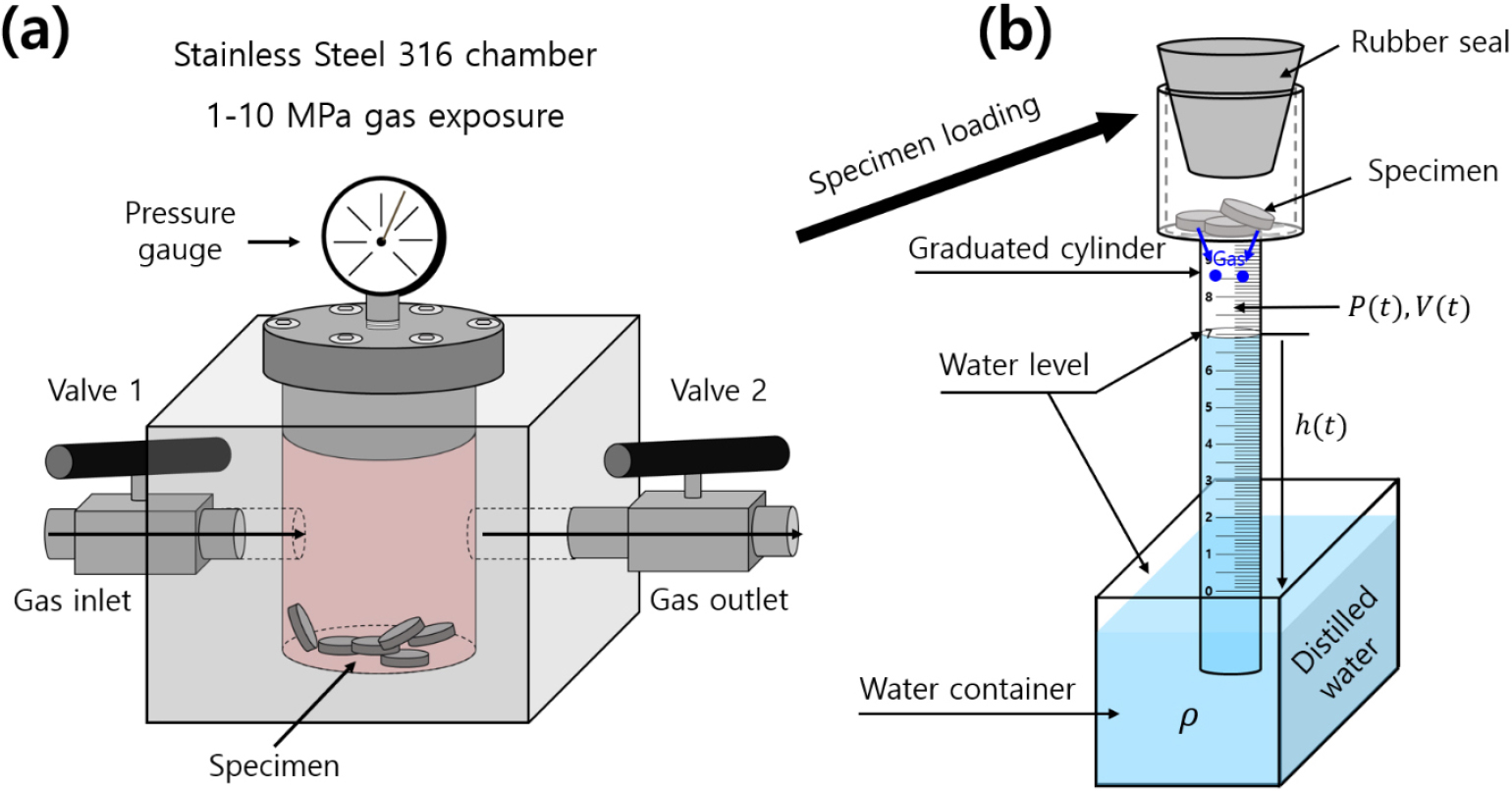
https://cdn.apub.kr/journalsite/sites/mrsk/2025-035-03/N0340350302/images/mrsk_2025_353_127_F1.jpg

Fig. 1.

Volumetric sensor system to measure the gas uptake and diffusivity emitted by a specimen after charging to HP gas. (a) Specimen charged to gas in a HP chamber. (b) After decompression in the chamber, the specimen was loaded into a graduated cylinder. The cylinder was partially immersed in a water container and gas emission measurements were performed. The blue circle in cylinder represents the gas emitted from the charged sample.

After charging to high-pressure gas and decompression, the specimen was placed in the upper air space of a graduated cylinder, as depicted in Fig. 1. The gas released from the specimen caused a gradual decrease in the water level within the cylinder. Consequently, the pressure (P) and volume (V) of the gas inside the cylinder varied with time.

The gas within the cylinder adheres to the ideal gas law, expressed as PV = nRT, where R is the gas constant (8.20544 × 10^-5 m³･atm/(mol･K)), T represents the gas temperature inside the cylinder, and n denotes the number of moles of gas released into the cylinder. The variations of pressure P(t) and volume V(t) of the gas in the cylinder can be described as follows⁸⁷⁾:

(1)

P (t) = P_{o} (t) - ρ g h (t), V (t) = V_{o} - V_{s} - V_{h} (t)

where $P_{o}$ represents the external pressure surrounding the cylinder, g is the gravitation acceleration, and ρ signifies the density of distilled water. The $h (t)$ describes the water level within the cylinder over time, while $V_{o}$ is the combined volume of gas and water inside the cylinder, measured relative to the water level in the container. $V_{h} (t)$ indicates the time-dependent volume of water in the cylinder, and $V_{s}$ represents the volume occupied by the sample.

The amount of gas released by the polymer specimen was quantified by tracking the water level position [ $V_{h} (t)$ ] over time. Consequently, the total moles of gas emitted [ $n (t)$ ] were calculated by measuring the total gas volume [ $V (t)$ ] in the graduated cylinder, which corresponds to the decrease in the water level, as expressed by the following⁸⁷⁾:

(2)

n (t) = \frac{P (t) V (t)}{R T (t)} = \frac{P (t) [V_{A} + V_{H} (t)]}{R T (t)} = \frac{P_{0} [1 + β (t)] [V_{A} + V_{H} (t)]}{R T_{0} [1 + α (t)]} ≅ \frac{P_{0}}{R T_{0}} [V_{A} + V_{H} (t) + V (t) (β (t) - α (t))] = n_{A} (t) + n_{H} (t), with, n_{A} (t) = \frac{P_{0}}{R T_{0}} V_{A}, n_{H} (t) = \frac{P_{0}}{R T_{0}} [V_{H} (t) + V (t) (β (t) - α (t))] α (t) = \frac{T (t) - T_{0}}{T_{0}}, β (t) = \frac{P (t) - P_{0}}{P_{0}}

Here, $T_{0}$ and $P_{0}$ represent the initial temperature and pressure of the gas in the cylinder, respectively. $V (t)$ is the total volume, consisting of the remaining initial air volume ( $V_{A}$ ) and the released gas volume [ $V_{h} (t)$ ], so that $V (t) = V_{A} + V_{H} (t)$ . $n_{A}$ denotes the initial mole number of air and $n_{H} (t)$ refers to the time-dependent mole number of gas corresponding to the increase in gas volume due to its release. Therefore, $n_{H} (t)$ was converted to the gas concentration, [ $C (t)$ emitted per unit mass from the specimen as :

(3)

C (t) [w t ∙ p p m] = n_{H} (t) [m o l] \times \frac{m_{Gas} [. g / mol]}{m_{sample} [. g]} \times 10^{6} = \frac{P_{0}}{R T_{0}} [V_{H} (t) + V (t) (β (t) - α (t))] [m o l] \times \frac{m_{H 2} [\frac{g}{m o l}]}{m_{sample} [. g]} \times 10^{6}

For instance, the molar mass of hydrogen gas, $m_{H 2}$ [g/mol] is 2.016 g/mol. The molar mass of nitrogen gas $m_{N 2}$ [g/mol] is 28.013 g/mol. $m_{s a m p l e}$ is the specimen mass. In Eqs. (2) and (3), the time-dependent mole number of gas, $n_{H} (t)$ , was converted to the gas mass concentration, [ $V (t)$ ], by the factor, $k = [\frac{m_{Gas}}{m_{sample}}]$ . $n_{H} (t)$ and $C (t)$ are affected by the fluctuations of temperature and pressure in the laboratory environments. To ensure precise measurements, it’s essential to compensate for these variations. This compensation can be achieved through automated programs according to Eq. (3). That is, the terms, $V (t) (β (t) - α (t))$ , indicates the volume change in the $V_{H} (t)$ , caused by the temperature and pressure variations. The compensation indicates the application of $V (t) (β (t) - α (t))$ calculation in Eq. (3). Thus, the insensitivity of the sensor to variations in temperature and pressure means the application of automatic compensation by the program.

The release of gas was tracked by monitoring changes in water level measurement using image processing algorithm via digital camera in front of the graduated cylinder. The procedure for obtaining the water level (emitted gas volume) from water level measurement is described in previous works.^5,83)

2.3. Manometric measurement of the released gas from charged polymers

Fig. 2 illustrates the schematic of the manometric measurement sequence used to determine the concentration and diffusivity of the released gas from specimen at 298 K. The setup includes a high-pressure chamber for the gas charging as shown in Fig. 2(a), a rectangular specimen container equipped with a commercial data logger with USB type and rubber seal in Fig. 2(b). The ELP sensors, which were used to measure pressure and temperature, are commercial data loggers capable of simultaneously recording both atmospheric pressure and temperature.

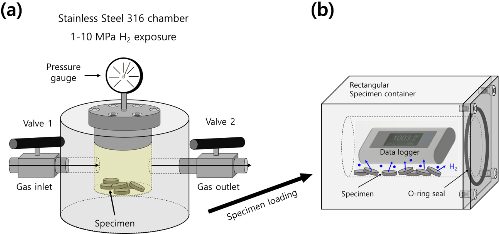
https://cdn.apub.kr/journalsite/sites/mrsk/2025-035-03/N0340350302/images/mrsk_2025_353_127_F2.jpg

Fig. 2.

Illustration of manometric sensor system for measuring gas uptake and diffusion coefficient from charged sample using a commercial pressure/temperature logger after high-pressure charging and decompression. (a) The sample charged to gas in the high-pressure chamber. (b) After decompression of the chamber, the charged sample loaded in the rectangular specimen container. Gas emission measurements were carried out using a data logger within the sample container. The blue circle in specimen container represents the gas emitted from charged sample.

After the charging and decompression in the stainless steel chamber, the specimen was transferred into the rectangular specimen container shown in Fig. 2(b). As the gas released from the sample, the pressure inside the vessel increased with elapsed time. Consequently, both the pressure (P) and temperature (T) of the gas within the specimen container changed as time progressed. The gas inside the container followed the ideal gas law: PV = nRT, R is the gas constant with 8.20544 × 10^-5 m³･atm/(mol･K), and n represents the number of moles of the released gas molecules inside the specimen container.

The mole number of gases emitted from charged specimen is obtained by measuring the increase in pressure [ $P (t)$ ] versus time by manometric measurement at a constant container volume. Thus, the total number of moles [ $n (t)$ ] obtained by measuring the increased gas pressure [ $P (t)$ due to emitted gas in the cylindrical container is described as follows^3,86):

(4)

n (t) = \frac{P (t) V_{0}}{R T (t)} = \frac{P (t) V_{0}}{R T (t)} = \frac{[P_{0} + Δ P (t)] V_{0}}{R T_{0} [1 + α (t)]} ≅ \frac{P_{0} V_{0} + Δ P (t) V_{0}}{R T_{0}} [1 - α (t)] = n_{0} + Δ n (t), with n_{0} = \frac{P_{0} V_{0}}{R T_{0}}, Δ n (t) = \frac{V_{0}}{R T_{0}} [Δ P (t) - α (t) P_{0} - α (t) Δ P (t)] α (t) = \frac{T (t) - T_{0}}{T_{0}}

where $T_{0}$ , $V_{0}$ and $P_{0}$ are the temperature, initial volume and initial pressure of the air at initial time inside the cylinder with the sample, respectively. $P (t)$ is the sum of remaining initial air pressure ( $P_{o}$ ) and time-varying released gas pressure [∆ $P (t)$ ] from specimen, i.e., $P (t) = P_{o} + △ P (t)$ , $n_{0}$ is remaining initial air mole, and ∆ $n (t)$ is the time-varying gas mole corresponding to gas pressure increase by the released gas. $α (t)$ is the change rate of temperature with respect to $T_{0}$ . Thus, ∆ $n (t)$ is transformed into the released gas concentration [∆ $C (t)$ ] per mass for specimen as⁸⁶⁾:

(5)

Δ C (t) [w t p p m] = Δ n (t) [m o l] \times \frac{m_{g} [\frac{g}{m o l}]}{m_{specimen} [g]} \times 10^{6} = \frac{V_{0}}{R T_{0}} [Δ P (t) - α (t) P_{0} - α (t) Δ P (t)] [m o l] \times \frac{m_{g} [\frac{g}{m o l}]}{m_{specimen} [g]} \times 10^{6}

where $m_{g}$ [g/mol] is molar mass of the gas used; for H₂, $m_{H 2}$ [g/mol] = 2.016 g/mol and for N₂, $m_{N 2}$ [g/mol] = 28.001 g/mol; and $m_{s p e c i m e n}$ is sample mass. First term, ∆ $P (t)$ in Eq. (5), is the increase in pressure that is emitted gas from sample. The second term, $- α (t) P_{0}$ , is the pressure change caused by temperature variation [ $α (t)$ ]. The third term, $- α (t) △ P (t)$ , is the pressure change due to both temperature variation [ $α (t)$ ] and pressure increase [∆ $P (t)$ ].

According to Eqs. (4) and (5), the time-varying gas mole, ∆ $n (t)$ , is transformed to gas mass concentration, [∆ $C (t)$ ], by $k : k = [\frac{m_{g}}{m_{specimen}}]$ . ∆ $n (t)$ and ∆ $C (t)$ are affected by both temperature and pressure variations. Thus, we have compensated for the variations caused by changes in temperature and pressure.

2.4. Analysis program for obtaining transport parameters

Released gas concentration from the gas-charged sample follows Fickian diffusion. Thus, the concentration of released gas, $C_{E} (t)$ , is calculated as follows^88,89):

(6)

C_{B} (t) / C_{\infty} = 1 - \frac{32}{π^{2}} \times [\sum_{n = 0}^{\infty} \frac{\exp \frac{- (2 n + 1)^{2} π^{2} D t}{l^{2}}] \times [\sum_{n = 1}^{\infty} \frac{\exp \{\frac{D β_{n}^{2} t}{ρ^{2}}\}}{β_{n}^{2}}]}{(2 n + 1)^{2}}] = 1 - \frac{32}{π^{2}} \times [\frac{\exp (- \frac{π^{2} D t}{l^{2}})}{1^{2}} + \frac{\exp (- \frac{3^{2} π^{2} D t}{l^{2}})}{3^{2}} + \dots, + \frac{\exp (- \frac{(2 n + 1)^{2} π^{2} D t}{l^{2}})}{(2 n + 1)^{2}} + \dots,] \times [\frac{\exp (- \frac{D β_{1}^{2} t}{ρ^{2}})}{β_{1}^{2}} + \frac{\exp (- \frac{D β_{2}^{2} t}{ρ^{2}})}{β_{2}^{2}} + \dots, + \frac{\exp (- \frac{D β_{n}^{2} t}{ρ^{2}})}{β_{n}^{2}} + \dots,]

where $β_{n}$ represents root of zeroth-order Bessel function, J₀(β_n). This equation corresponds to solution of Fick’s second diffusion equation for a cylindrical shaped specimen. C_E(t = 0) = 0 and C_E(t = ¥) = $C_{\infty}$ is saturated gas concentration at infinite time, indicating total gas uptake (emission content). D is the gas diffusivity. $l$ and 𝜌 are thickness and radius of cylindrical sample, respectively.

For the exact calculation by Eq. (6), many terms in the product of two summations are contained. Therefore, dedicated analysis program is developed that calculates precisely $C_{\infty}$ and D. With an analysis program based on an optimization algorithm,⁹⁰⁾ we accurately calculate $C_{E} (t)$ and D from the measured result by solving Eq. (6).

3. Results and Discussion

3.1. Volumetric measurement

After decompressing a specimen charged with corresponding gas under high pressure, the released gas concentration and diffusivity were determined using the VM method with a graduated cylinder (Fig. 1). The water level in VM method is measured by employing image processing algorithm and a digital camera.⁸³⁾Fig. 3 displays the measured and fitted results for five gases in cylindrical EPDM determined from the water level measurement by VM. The left sides of Fig. 3(a-e) show corresponding emitted gas volume (blue filled circle) transferred from water level measurement. The right sides of Fig. 3(a-e) represent corresponding gas emission data (black open square). The diffusion parameters, D and $C_{\infty}$ , are derived using an analysis program by Eq. (6). The blue line in right side is fitted result using Eq. (6), with diffusivity (D) and the total gas uptake (C_∞) marked by a blue arrow. As shown in Fig. 3(a-e), single mode gas emission behaviors for all gases in EPDM were observed under time-dependent gas emission measurement. The single-mode gas emission in EPDM results from gas diffusion into the amorphous phase.

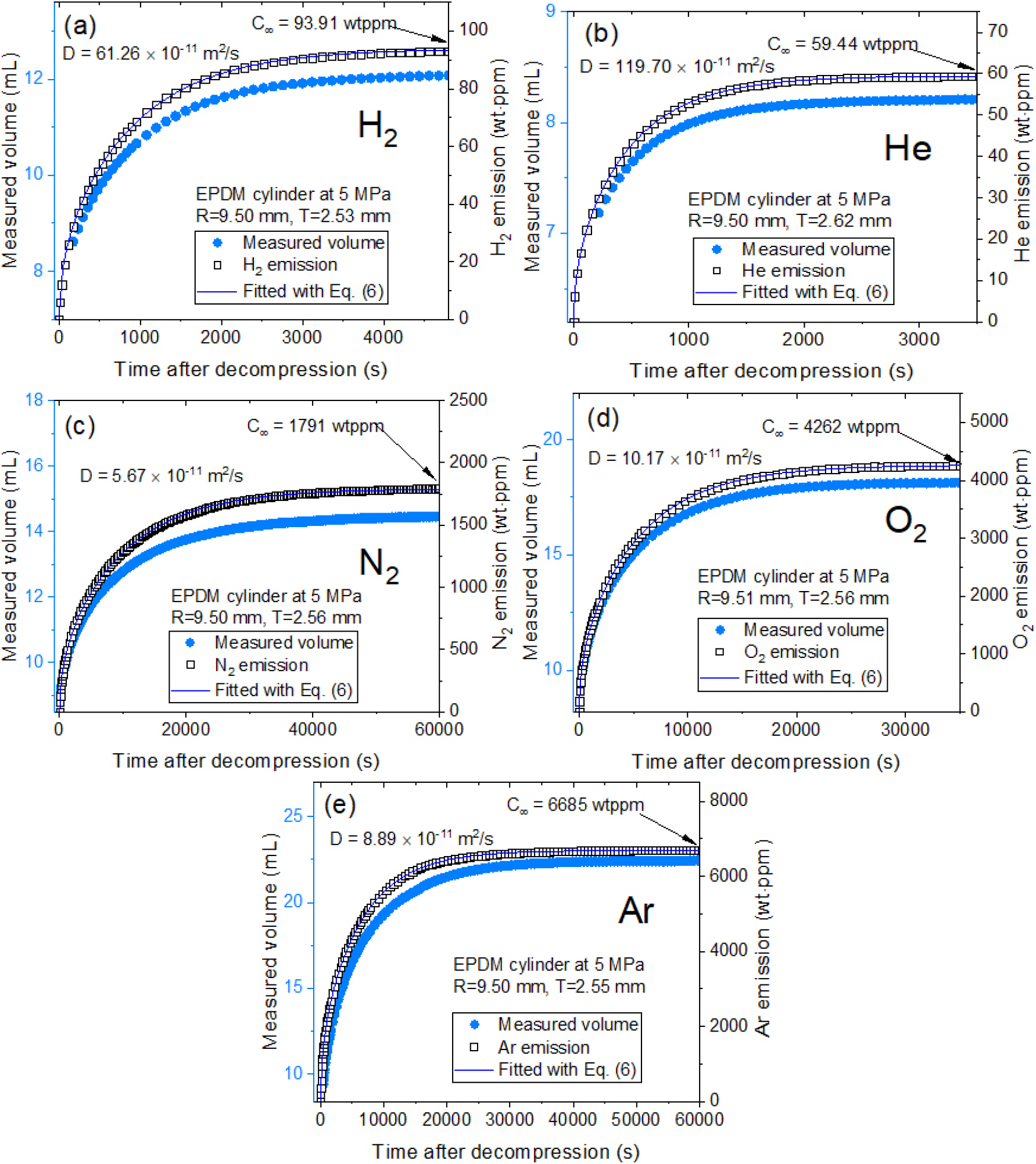
https://cdn.apub.kr/journalsite/sites/mrsk/2025-035-03/N0340350302/images/mrsk_2025_353_127_F3.jpg

Fig. 3.

Gas uptake and diffusivity determined from five gases in a cylindrical EPDM specimen by volumetric measurement using image processing algorithm and a digital camera. (a-e): Measured gas volume (blue filled circle) transformed from the measured water level and emitted gas emission (black open square) transferred from measured gas volume in unit of wt･ppm. The blue line represents the fitted data using Eq. (6), with gas diffusivity the total gas uptake marked by a blue arrow. Here, R is radius of cylindrical specimen. T is thickness of cylindrical specimen.

3.2. Manometric measurement

After decompressing a specimen charged with hydrogen under high pressure, the released gas concentration and diffusivity were determined using the MM method for specimen loaded in the cylinder-shaped container (Fig. 2). The water level in MM method is measured by employing commercial USB-type manometer. Fig. 4(a-e) display the measured and fitted results for five gases in cylindrical EPDM determined from the water level measurement by MM. The left and right sides of Fig. 4(a-e) represent emitted gas pressure and gas emission content, respectively. The right sides of Fig. 4(a-e) represent the diffusion parameters, D and $C_{\infty}$ , derived using a diffusion analysis program by Eq. (6). The blue line in right side is fitted data using Eq. (6), with gas diffusivity and the total gas uptake marked by a blue arrow. In similarity with Fig. 3, a single-mode gas emission behaviors for all gases in EPDM were also observed under time-varying gas emission measurement in Fig. 4.

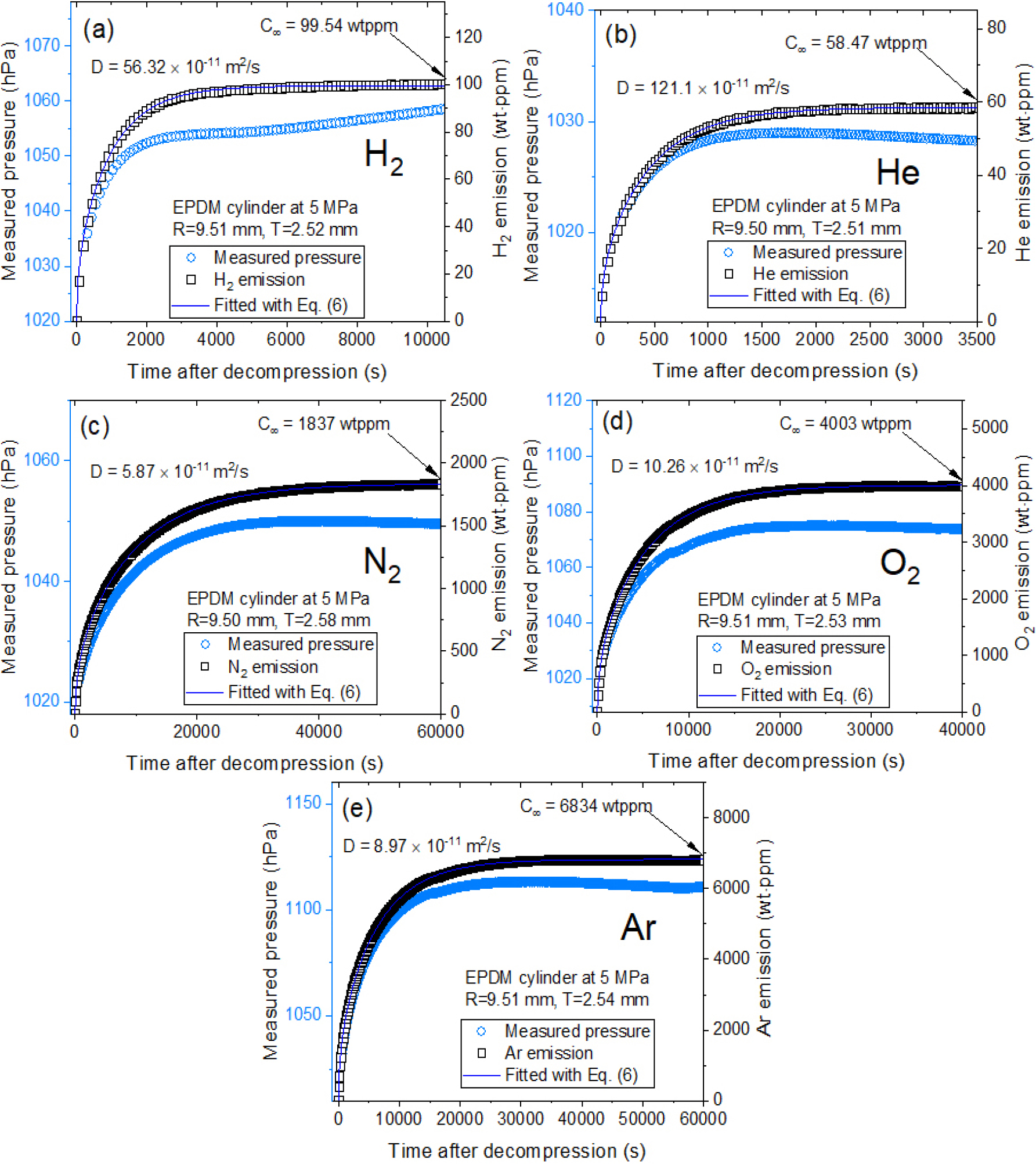
https://cdn.apub.kr/journalsite/sites/mrsk/2025-035-03/N0340350302/images/mrsk_2025_353_127_F4.jpg

Fig. 4.

Gas uptake and diffusivity determined from five gases in a cylindrical EPDM specimen by manometric measurement using data logger. (a-e): Measured gas pressure (blue filled circle) and emitted gas emission (black open square) transferred from measured gas pressure in unit of wt･ppm. The blue line represents the fitted data using Eq. (6), with gas diffusivity the total gas uptake marked by a black arrow. The difference in patterns between the measured pressure and H₂ emission is due to temperature/pressure compensation applied using Eq. (6). Here, R is radius of cylindrical specimen. T is thickness of cylindrical specimen.

Fig. 4. Gas uptake and diffusivity determined from five gases in a cylindrical EPDM specimen by manometric measurement using data logger. (a-e): Measured gas pressure (blue filled circle) and emitted gas emission (black open square) transferred from measured gas pressure in unit of wt･ppm. The blue line represents the fitted data using Eq. (6), with gas diffusivity the total gas uptake marked by a black arrow. The difference in patterns between the measured pressure and H₂ emission is due to temperature/pressure compensation applied using Eq. (6). Here, R is radius of cylindrical specimen. T is thickness of cylindrical specimen.

Moreover, solubility (S) is obtained from gas uptake versus pressure from Figs. 3, 4 as follows^84,91,92,93):

(7)

S [\frac{m o l}{m^{3} \cdot M P a}] = \frac{(C_{\infty} / pressure) [\frac{w t ∙ p p m}{M P a}] \times 10^{6} \times d [\frac{g}{m^{3}}]}{m_{g} [\frac{g}{m o l}]}

$m_{g}$ is molar mass of the charged gas and $d$ is density of the sample. The solubility and diffusivity in two sensors determined for H₂, He, N₂, O₂ and Ar gases in EPDM sample are shown in Tables 1 and 2, respectively.

Table 1.

Summary for solubility and diffusivity of five gases measured by VM and MM in EPDM.

Sensing method	Solubility [mol/m³･MPa]					Diffusion coefficient [× 10^-11 m²/s]
Sensing method	H₂	He	N₂	O₂	Ar	H₂	He	N₂	O₂	Ar
VM	8.55	3.24	13.94	24.45	30.42	61.26	119.70	5.67	10.17	8.89
MM	9.07	3.18	14.30	22.97	31.09	56.32	121.10	5.87	10.26	8.97

Table 2.

Performance comparisons for two sensor systems with volumetric and manometric methods.

Performance	Volumetric measurement	Manometric measurement
Sensitivity	16.43 wt･ppm/mL	11.96 wt･ppm/hPa
Resolution	0.08 wt･ppm	0.12 wt･ppm
Stability	0.2 %	0.2 %
Measuring range	Max. 1400 wt･ppm	Max. 1500 wtppm
Response time	~1 s	~1 s
FOM	0.4 %	0.7 %

In Table 1, the solubility and diffusion coefficient in two specimens for two sensors have 10 % relative expanded uncertainty for measured value. The solubility and diffusion coefficient results obtained from both the VM and MM were consistent within the estimated relative uncertainty.

3.3. Performance comparison between volumetric and manometric gas sensors

We have evaluated the performance of two gas sensing system using volumetric image sensor and manometric data logger sensor. The results of the performance tests are represented in Table 2, covering sensitivity, resolution, stability, measurable range, response time and figure of merit (FOM). Sensitivity in VM and MM sensor is defined as the mass concentration change relative to the change in measured volume and measured pressure, respectively. The obtained sensitivities were 16.43 wt･ppm/mL for the VM sensor and 11.96 wt･ppm/hPa for the MM sensor. A sensor with higher sensitivity typically provides better resolution. For the VM sensor, the resolution is reflected by the minimum measurable volume of 0.005 mL, corresponding to a mass concentration of 0.08 wt･ppm. For the MM sensor, the resolution is reflected by the minimum measurable pressure of 0.01 hPa, corresponding to a mass concentration of 0.12 wt･ppm. To improve resolution further, it is possible to reduce the inner volume of the graduated cylinder and the sample container or increase the number of specimens. This adjustment would lead to better sensitivity and resolution.

The stability of two sensor systems is quantified by the standard deviation of measurements taken over 36 h after gas emission from the specimen ceased. This was found to be less than 0.2 % of the mass concentration for both sensors. The measurable range in VM sensor is obtained as the maximum allowable concentration per mass of specimen within graduated cylinder with inner volumes. The measurable range in MM sensor is determined as the maximum allowable concentration per mass of specimen within a specimen container with inner volumes. For both the sensors, the measurable range was 1400 wt･ppm for VM sensor and 1500 wt･ppm for MM sensor, which can be adjusted by varying the sample mass, cylinder volume and specimen container volume. The gas sensor’s volume and pressure response are almost instantaneous, occurring within ~1 second of gas emission. The FOM is defined as the standard deviation between measured data and the theoretical value calculated using Eq. (3). An FOM value is below 0.4 % for VM sensor and 0.7 % for MM sensor, indicating good agreement between the measured and theoretical values. Based on the performance testing, the specifications (sensitivity, resolution and FOM) of VM sensor are superior to MM sensor.

4. Conclusion

Gas sensors are crucial for ensuring safety and protecting property in gas-related facilities. We have developed two gas sensing systems that utilize volumetric measurements with a graduated cylinder, coupled with an image processing algorithm and a digital camera. The variation in the water level, observed through pixel shifts in the graduated cylinder, is directly linked to changes in water volume caused by the released gas, allowing for precise measurement of gas concentration. By integrating a diffusion-permeation analysis program, this volumetric image-based gas sensor is capable of detecting not only gas concentrations but also solubility/diffusivity from gas-charged specimens under high-pressure conditions.

A straightforward manometric gas sensor was also developed for characterizing gas behavior. The method relies on pressure measurements within a gas charged sample container, utilizing a commercial data logger. The system measures the pressure increase caused by the gas released from high-pressure polymer samples, enabling the determination of gas concentration and solubility/diffusivity by a diffusion analysis program.

The two portable gas sensor systems showcased several key performance metrics: a low detection limit for gas content, a measurable range of up to 1500 wt･ppm, stability of 0.2 %, and a rapid response time within one second. Additionally, the sensors’ insensitivity to temperature and pressure fluctuations made them highly reliable for gas detection. The sensing systems, utilizing both volumetric and manometric measurements, successfully demonstrated real-time monitoring and characterization of pure gases such as H₂, He, N₂, O₂ and Ar. The sensors effectively measured gas uptake and diffusivity, considering influencing factors and calculating expanded uncertainty. In conclusion, the main features of the two developed gas sensing methods are summarized as follows:

(1) Cost-effective and simple techniques: The two methods provide affordable and straightforward solutions for evaluating gas uptake and diffusion coefficient in gas charged polymers under high-pressure.

(2) Stability against temperature and pressure variations: Both methods are stable under fluctuations in temperature and pressure. Two sensors are independent of a specimen sizes, shapes and gas types.

(3) Adjustable sensitivity and range: The volumetric and manometric methods offer flexible sensitivity, resolution, and measurement range, allowing for customization based on specific application requirements.

(4) No chemical interaction: Both sensing methods function without any interaction between the gas molecules and the sensor, ensuring accurate measurements without altering the composition of the gas.

(5) Visible gas release monitoring: The volumetric method provides visual gas monitoring of gas release by changes in water level.

These two complementary sensing methods are highly effective for measuring gas transport properties of sealing elastomers and can be applied to assess the permeation characteristics of rubber materials and O-rings under high-pressure conditions. They are particularly well-suited for applications in hydrogen fueling stations. The results from both sensing methods demonstrated consistent measurements of gas solubility and diffusivity, with a comprehensive review of their characteristics and performance, ensuring their reliability and applicability in the field.

Author Information

Ji Hun Lee

Researcher, Hydrogen Energy Group, Korea Research Institute of Standards and Science

Sang Koo Jeon

Senior Researcher, Hydrogen Energy Group, Korea Research Institute of Standards and Science

References

Z. Wang, L. Zhu, J. Zhang, J. Wang, X. Cui, X. Chen, W. Liu, H. Ma, J. Wang and W. Yan, Sens. Actuators B Chem., 418, 136276 (2024).

10.1016/j.snb.2024.136276

S. D. Lawaniya, S. Kumar, Y. Yu, Y. K. Mishra and K. Awasthi, Metal oxide-polymer composites for gas-sensing applications, p. 107-150, in Complex and Composite Metal Oxides for Gas VOC and Humidity Sensors : Volume 1: Fundamentals and Approaches (eds. B. C. Yadav and P. Kumar), Elsevier, Amsterdam, Netherlands (2024).

10.1016/B978-0-323-95385-6.00012-X

J. K. Jung, I. G. Kim, K. S. Chung and U. B. Baek, Mater. Chem. Phys., 267, 124653 (2021).

10.1016/j.matchemphys.2021.124653

J. K. Jung and J. H. Lee, Sci. Rep., 14, 1967 (2024).

J. Li, Y. Li and W. Zeng, Sens. Actuators A Phys., 365, 114890 (2024).

10.1016/j.sna.2023.114890

Y. Yang, S. Zheng, X. Fu and H. Zhang, Optik, 158, 602 (2018).

10.1016/j.ijleo.2017.12.151

P. Mohapatra, S. Panigrahi and J. Amamcharla, J. Food Meas. Charact., 9, 121 (2015).

10.1007/s11694-014-9200-9

M. Wenger, R. Waller, V. R. H. Lorentz, M. Marz and M. Herold, in Proceedings of IECON 2014 - 40th Annual Conference of the IEEE Industrial Electronics Society (IEEE, Dallas, TX, USA, 2014) p.5654.

H. M. Kang, M. C. Choi, J. H. Lee, Y. M. Yun, J. S. Jang, N. K. Chung, S. K. Jeon, J. K. Jung, J. H. Lee, J. H. Lee, Y. W. Chang and J. W. Bae, Polymers, 14, 1151 (2022).

10.3390/polym1406115135335482PMC8949588

J. K. Jung, I. G. Kim and K. T. Kim, Curr. Appl. Phys., 21, 43 (2021).

A. Sony, K. Acharjya, K. Sharma and N. Beemkumar, E3S Web Conf., 540, 11001 (2024).

10.1051/e3sconf/202454011001

S. E. Kayacık, A. H. Schrotenboer, E. Ursavas and I. F. A. Vis, Sustain. Energy Grids Netw., 38, 101394 (2024).

10.1016/j.segan.2024.101394

I. Amez, B. Castells, D. León and R. Paredes, Fuel, 381, 133663 (2025).

10.1016/j.fuel.2024.133663

M. Wu, L. Bai, F. Deng, J. He, K. Song and H. Li, Coord. Chem. Rev., 523, 216259 (2025).

10.1016/j.ccr.2024.216259

M. Tang, C. Qin, X. Sun, M. Li, Y. Wang, J. Cao and Y. Wang, Appl. Phys. A, 130, 741 (2024).

10.1007/s00339-024-07905-w

J. K. Jung, I. G. Kim, K.-T. Kim, U. B. Baek and S. H. Nahm, Curr. Appl. Phys., 26, 9 (2021).

10.1016/j.cap.2021.03.005

A. Tom, D. K. Singh, V. K. Shaw, P. V. Abhijith, S. Sajana, P. S. Kirandas, V. Dixit, V. Kamble, S. P. Pai and D. Jaiswal-Nagar, Rev. Sci. Instrum., 95, 085003 (2024).

10.1063/5.020294039145696

R. Venkatesan, R. Harun, H. M. Yusoff and M. A. Razak, Process Saf. Prog., 43, S161 (2024).

10.1002/prs.12590

A. A. Malik, R. Rusli, S. Nazir, R. H. Wong and U. Arshad, Process Saf. Prog., 43, S35 (2024).

10.1002/prs.12567

J.-N. Lu, Y. Huang, Y.-S. Xia, L.-Z. Dong, L. Zhang, J.-J. Liu, L.-G. Xie, J. Liu and Y.-Q. Lan, Carbon Energy, 6, e396 (2024).

H. Kang, J. Bae, J. Lee, Y. Yun, S. Jeon, N. Chung, J. Jung, U. Baek, J. Lee, Y. Kim and M. Choi, Polymers, 16, 1065 (2024).

10.3390/polym1608106538674985PMC11054514

J.-K. Jung, K.-T. Kim, N.-K. Chung, U.-B. Baek and S.-H. Nahm, Polymers, 14, 1468 (2022).

10.3390/polym1407146835406341PMC9003005

Y. Wang, Y. Pang, H. Xu, A. Martinez and K. S. Chen, Energy Environ. Sci., 15, 2288 (2022).

10.1039/D2EE00790H

H. Fujiwara, H. Ono, K. Onoue and S. Nishimura, Int. J. Hydrog. Energy, 45, 29082 (2020).

10.1016/j.ijhydene.2020.07.215

A. Fujisawa, S. Kinoshita, S.-I. Miura, S. Nakao, F. Suzuki and K. Yamashita, Kobe Steel Eng. Rep., 70, 3 (2020).

J. K. Jung, Y. I. Moon, K. S. Chung and K.-T. Kim, Macromol. Res., 28, 596 (2020).

10.1007/s13233-020-8080-6

J. S. Jang and N. K. Chung, in Proceedings of the ASME 2020 Pressure Vessels and Piping Conference (Virtual Conference, August 2020), p. V001T01A041.

I. Profatilova, F. Fouda-Onana, M. Heitzmann, T. Bacquart, A. Morris, J. Warren, F. Haloua and P.-A. Jacques, Int. J. Hydrog. Energy, 65, 837 (2024).

10.1016/j.ijhydene.2024.04.055

N. C. Menon, A. M. Kruizenga, K. J. Alvine, C. San Marchi, A. Nissen and K. Brooks, in Proceedings of the Pressure Vessels and Piping Conference (Vancouver, British Columbia, Canada, July 2016), p. V06BT06A037.

Y. I. Moon, J. K. Jung, G. H. Kim and K. S. Chung, Phys. B, 608, 412870 (2021).

10.1016/j.physb.2021.412870

S. U. Zhanguo, W. Zhang, A. Abdulwahab, S. Saleem, Y. Yao, A. Deifalla and M. Taghavi, Process Saf. Environ. Prot., 173, 317 (2023).

10.1016/j.psep.2023.03.015

J. K. Jung, J. H. Lee, S. K. Jeon, U. B. Baek, S. H. Lee, C. H. Lee and W. J. Moon, Polymers, 15, 162 (2023).

10.3390/polym1501016236616510PMC9824334

J. K. Jung, U. B. Baek, S. H. Lee, M. C. Choi and J. W. Bae, J. Polym. Sci., 61, 460 (2023).

10.1002/pol.20220494

B.-L. Choi, J.-K. Jung, U.-B. Baek and B.-H. Choi, Polymers, 14, 861 (2022).

10.3390/polym1405086135267684PMC8912785

C. H. Lee, J.-K. Jung, S. K. Jeon, K. S. Ryu and U. B. Baek, Journal of Magnetics, 22, 478 (2017).

10.4283/JMAG.2017.22.3.478

B. Flamm, C. Peter, F. N. Büchi and J. Lygeros, Appl. Energy, 281, 116031 (2021).

10.1016/j.apenergy.2020.116031

W. Kuang, W. D. Bennett, T. J. Roosendaal, B. W. Arey, A. Dohnalkova, G. Petrossian and K. L. Simmons, Tribol. Int., 153, 106627 (2021).

10.1016/j.triboint.2020.106627

J.-H. Lee, Y.-W. Kim and J.-K. Jung, Polymers, 15, 4019 (2023).

10.3390/polym1519401937836068PMC10575446

J. H. Lee, Y. W. Kim, D. J. Kim, N. K. Chung and J. K. Jung, Polymers, 16, 280 (2024).

10.3390/polym1602028038276688PMC10821381

J. H. Lee, Y. W. Kim, N. K. Chung, H. M. Kang, W. J. Moon, M. Chan Choi and J. K. Jung, Polymer, 311, 127552 (2024).

10.1016/j.polymer.2024.127552

C. H. Lee, J. K. Jung, K. S. Kim and C. J. Kim, Sci. Rep., 14, 5319 (2024).

10.1038/s41598-024-81931-939638849PMC11621780

J. K. Jung, J. H. Lee, J. S. Jang, N. K. Chung, C. Y. Park, U. B. Baek and S. H. Nahm, Sci. Rep., 12, 3328 (2022).

10.1038/s41598-022-07321-135228634PMC8885926

Y. Moon, H. Lee, J. Jung and H. Han, Sci. Rep., 13, 7846 (2023).

10.1038/s41598-023-34565-237188716PMC10185497

G.-H. Kim, Y.-I. Moon, J.-K. Jung, M.-C. Choi and J.-W. Bae, Polymers, 14, 155 (2022).

10.3390/polym1401015535012180PMC8747209

J. K. Jung, C. H. Lee, U. B. Baek, M. C. Choi and J. W. Bae, Polymers, 14, 592 (2022).

10.3390/polym1403059235160581PMC8839649

C. Liu, R. Zhang, L. Tian, C. Wang, X. Xu, Y. Pei and L. Yuxing, Nat. Gas Ind., 42, 145 (2022).

D. B. Smith, B. J. Frame, L. M. Anovitz and C. Makselon, in Proceedings of the Pressure Vessels and Piping Conference (Vancouver, British Columbia, Canada, July 2016), p. V06BT06A036.

Y.-S. Chou and J. W. Stevenson, J. Power Sources, 191, 384 (2009).

10.1016/j.jpowsour.2009.02.052

G. Li, J. Zhang, J. Chai, Z. Ni and Y. Yan, Int. J. Hydrog. Energy, 89, 738 (2024).

10.1016/j.ijhydene.2024.09.361

S. Yuan, S. Zhang, J. Wei, Y. Gao, Y. Zhu and H. Wang, Int. J. Hydrog. Energy, 91, 555 (2024).

10.1016/j.ijhydene.2024.10.066

S. K. Jeon, J. K. Jung, N. K. Chung, U. B. Baek and S. H. Nahm, Polymers, 14, 2233 (2022).

10.3390/polym1411223335683906PMC9182773

G. Theiler, N. C. Murillo and A. Hausberger, Lubricants, 12, 233 (2024).

10.3390/lubricants12070233

R. Checchetto, M. Scarpa, M. G. De Angelis and M. Minelli, J. Membr. Sci., 659, 120768 (2022).

G. J. Pavani, S. A. Pavani and C. A. Ferreira, Iran. Polym. J., 30, 583 (2021).

10.1007/s13726-021-00915-y

D. Brown, S. Neyertz, M. J. T. Raaijmakers and N. E. Benes, J. Membr. Sci., 577, 113 (2019).

10.1016/j.memsci.2019.01.039

G. Sun, C. Wang, J. Jia, H. Zhang, Y. Hu, Y. Liu and D. Zhang, J. Electron. Mater., 53, 3426 (2024).

10.1007/s11664-024-11146-1

J.-H. Lo, K. M. Smits, Y. Cho, G. P. Duggan and S. N. Riddick, Environ. Pollut., 341, 122810 (2024).

10.1016/j.envpol.2023.12281037925008

S. A. Sadovnikov, S. V. Yakovlev, N. S. Kravtsova, O. A. Romanovskii and D. A. Tuzhilkin, Sens. Int., 6, 100307 (2025).

10.1016/j.sintl.2024.100307

J. Meng, S. Balendhran, Y. Sabri, S. K. Bhargava and K. B. Crozier, Microsyst. Nanoeng., 10, 74 (2024).

10.1038/s41378-024-00697-238855359PMC11156923

H. Schlicke, R. Maletz, C. Dornack and A. Fery, Small, 20, 2403502 (2024).

10.1002/smll.20240350239291897PMC11600690

B. Molleman, E. Alessi, F. Passaniti and K. Daly, Inf. Process. Agric., 11, 573 (2024).

10.1016/j.inpa.2023.11.001

S.-K. Kwon, J.-N. Kim, H.-G. Byun and H.-J. Kim, Electrochem. Commun., 169, 107834 (2024).

10.1016/j.elecom.2024.107834

M. Eshkobilova, Z. Smanova, J. Begimqulov, S. Suvankulov and E. Abdurakhmanov, AIP Conf. Proc., 3244, 050007 (2024).

10.1063/5.0242048

X. Zhang, B. Ojha, H. Bichlmaier, I. Hartmann and H. Kohler, Sensors, 23, 4679 (2023).

10.3390/s2310467937430592PMC10222192

P. Rodlamul, S. Tamura and N. Imanaka, Bull. Chem. Soc. Jpn., 92, 585 (2019).

10.1246/bcsj.20180284

W. Jang, J.-S. Park, K.-W. Lee and Y. Roh, Micro Nano Syst. Lett., 6, 7 (2018).

10.1186/s40486-018-0069-y

R. Xie, S. Guan and Z. Tan, Opt. Commun., 574, 131105 (2025).

10.1016/j.optcom.2024.131105

Y. Zhang, M. Wang, P. Yu and Z. Liu, Sensors, 22, 7949 (2022).

10.3390/s2220794936298300PMC9611617

A. Yarai and T. Nakanishi, Rev. Sci. Instrum., 75, 3237 (2004).

10.1063/1.1791338

W. M. Seleka, K. E. Ramohlola, K. D. Modibane and E. Makhado, Int. J. Hydrog. Energy, 68, 940 (2024).

10.1016/j.ijhydene.2024.04.240

S. R. Mishra, V. Gadore and M. Ahmaruzzaman, Mater. Lett., 359, 135946 (2024).

10.1016/j.matlet.2024.135946

A. Asilian and S. M. Zanjani, Majlesi J. Electr. Eng., 18, 21 (2024).

J. K. Jung, I. G. Kim, K. S. Chung, Y.-I. Kim and D. H. Kim, Sci. Rep., 11, 17092 (2021).

10.1038/s41598-021-96266-y34429450PMC8385037

J. K. Jung, I. G. Kim, K. S. Chung and U. B. Baek, Sci. Rep., 11, 4859 (2021).

10.1038/s41598-021-83692-133649367PMC7921585

J. K. Jung, K.-T. Kim and K. S. Chung, Mater. Chem. Phys., 276, 125364 (2022).

10.1016/j.matchemphys.2021.125364

J. K. Jung, I. G. Kim, K. T. Kim, K. S. Ryu and K. S. Chung, Polym. Test., 93, 107016 (2021).

10.1016/j.polymertesting.2020.107016

F. Hardoyono and K. Windhani, Flavour Fragr. J., 38, 451 (2023).

10.1002/ffj.3759

Z. Huang, W. Yang, Y. Zhang, J. Yin, X. Sun, J. Sun, G. Ren, S. Tian, P. Wang and H. Wan, Anal. Chem., 96, 17960 (2024).

10.1021/acs.analchem.4c0256139445613

A. Hinojo, E. Lujan, J. Abella and S. Colominas, Fusion Eng. Des., 204, 114483 (2024).

10.1016/j.fusengdes.2024.114483

J. K. Jung, I. G. Kim, S. K. Jeon and K. S. Chung, Rubber Chem. Technol., 94, 688 (2021).

10.5254/rct.21.79880

X. Zhu, W. Ahmed, K. Schmidt, R. Barroso, S. J. Fowler and C. F. Blanford, IEEE Trans. Instrum. Meas., 73, 1 (2024).

10.1109/TIM.2024.3485428

Y. R. Shaltaeva, B. I. Podlepetsky and V. S. Pershenkov, Eur. J. Mass Spectrom., 23, 217 (2017).

10.1177/146906671772079529028397

J. H. Lee and J. K. Jung, Sensors, 24, 7699 (2024).

10.3390/s2423769939686236PMC11645017

J. K. Jung, I. G. Kim, S. K. Jeon, K.-T. Kim, U. B. Baek and S. H. Nahm, Polym. Test., 99, 107147 (2021).

10.1016/j.polymertesting.2021.107147

J. K. Jung, J. H. Lee, S. K. Jeon, N. H. Tak, N. K. Chung, U. B. Baek, S. H. Lee, C. H. Lee, M. C. Choi, H. M. Kang, J. W. Bae and W. J. Moon, Int. J. Mol. Sci., 24, 2865 (2023).

10.3390/ijms2403286536769186PMC9917398

J. K. Jung, K.-T. Kim and U. B. Baek, Curr. Appl. Phys., 37, 19 (2022).

J. K. Jung, Polymers, 16, 723 (2024).

J. Crank, The Mathematics of Diffusion, Clarendon Press, Oxford, UK (1979).

A. Demarez, A. G. Hock and F. A. Meunier, Acta Metall., 2, 214 (1954).

10.1016/0001-6160(54)90162-5

J. A. Nelder and R. Mead, Comput. J., 7, 308 (1965).

10.1093/comjnl/7.4.308

J. K. Jung, J. H. Lee, Y. W. Kim and N. K. Chung, Sens. Actuators B Chem., 418, 136240 (2024).

10.1016/j.snb.2024.136240

J. K. Jung, C. H. Lee, M. S. Son, J. H. Lee, U. B. Baek, K. S. Chung, M. C. Choi and J. W. Bae, Polymers, 14, 700 (2022).

10.3390/polym1404070035215613PMC8879493

J. K. Jung, K. T. Kim, U. B. Baek and S. H. Nahm, Polymers, 14, 756 (2022).

10.3390/polym1404075635215669PMC8874465

Korean Journal of Materials Research ISSN:1225-0562(Print) 2287-7258(Online) 한국재료학회지

Preview

Development of Gas Sensors for Measuring Gas Emission and Diffusion Coefficient in Gas Charged EPDM Polymer Using Volumetric and Manometric Analysis

ABSTRACT

MAIN

Fig. 1.

(1)

(2)

(3)

Fig. 2.

(4)

(5)

(6)

Fig. 3.

Fig. 4.

(7)

Table 1.

Summary for solubility and diffusivity of five gases measured by VM and MM in EPDM.

Table 2.

Performance comparisons for two sensor systems with volumetric and manometric methods.

Author Information

References